Trajectory Analysis & Optimization UI for Bipedal Robots (Real-Time Kinematics & Visualization)

Overview

The Trajectory Analysis & Optimization UI is a robust, user-friendly platform designed for real-time analysis and optimization of bipedal robot motion trajectories. Built to handle the demands of real-world exoskeleton and bipedal robot experiments, this UI empowers researchers and engineers to:

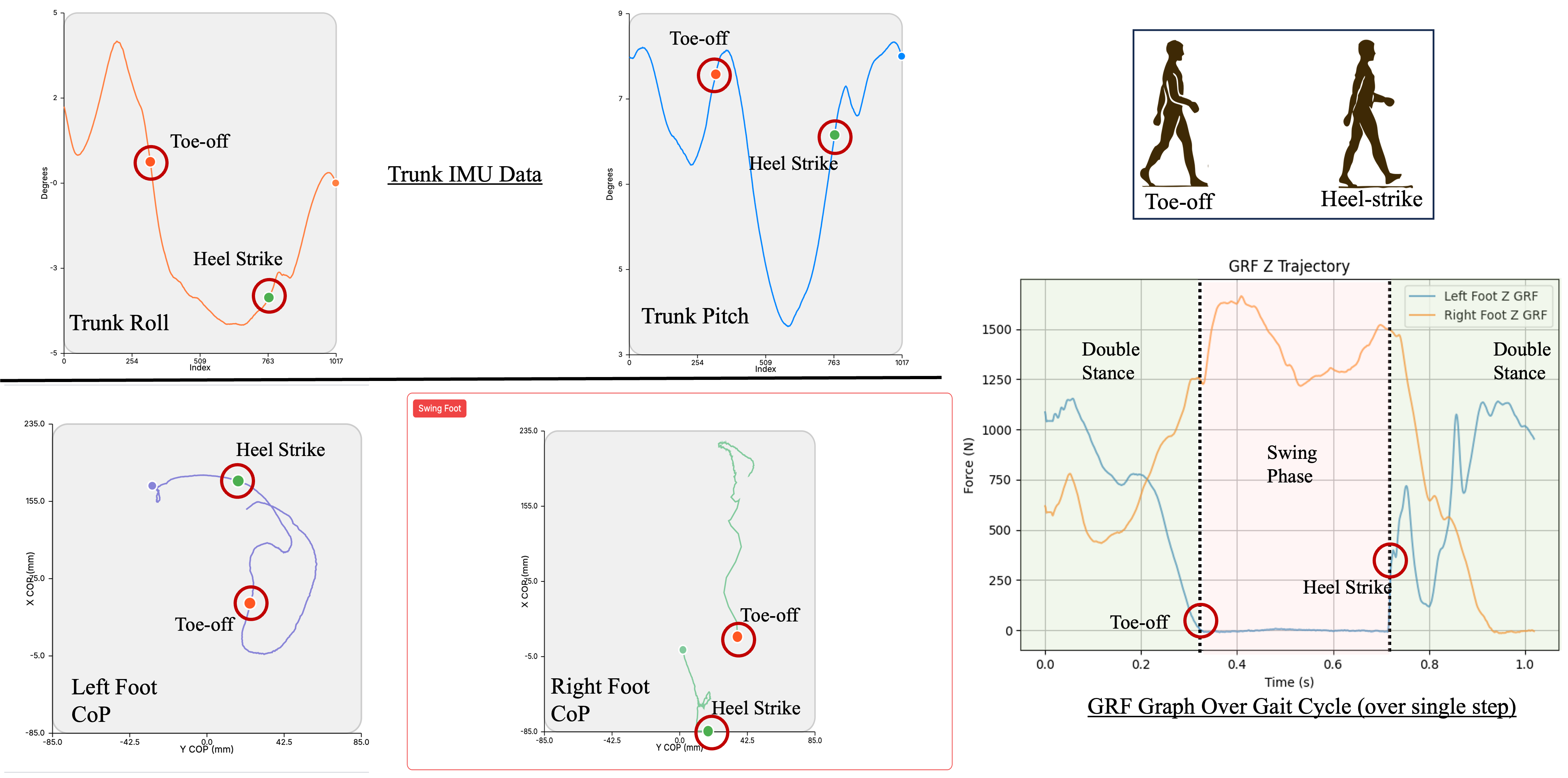
• Seamlessly analyze joint angle and sensor data in a user-friendly way
• Visualize complex trajectories from real-world experiments
• Modify trajectories in real-time using both forward and inverse kinematics
• Incorporate immediate user feedback for rapid iteration
• Efficiently process and visualize massive datasets (e.g., 6,300,000+ data points per minute)

Key Features

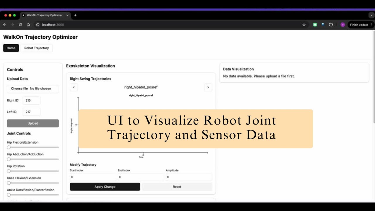
• User-Friendly Data Analysis: Intuitive interface for exploring joint angles, sensor data, and kinematic states.
• Real-Time Trajectory Visualization: Instantly plot and inspect trajectories from exoskeleton/bipedal robot experiments.
• Kinematics Integration: Modify and optimize trajectories using both forward and inverse kinematics, with immediate visual feedback.
• Rapid Testing & Iteration: Quickly test new trajectories and incorporate user feedback for efficient optimization.
• Scalable Data Handling: Designed to process and visualize millions of data points per minute without lag.
• 3D Robot Visualization: Interactive Meshcat viewer for real-time robot pose and trajectory visualization.

Technical Deep Dive

Data Pipeline

1. Data Ingestion

• CSV Upload: Users upload trajectory or sensor CSV files via the UI.
• Backend Parsing: The backend (backend/routes/upload.py, backend/services/data_processor.py) parses and standardizes the data, handling both single-level and multi-level CSV headers.
• State Segmentation: The pipeline identifies gait phases (e.g., right/left swing) using state columns, extracting relevant sequences for analysis.

2. Data Processing

• Standardization: Columns are mapped to canonical names (e.g., 'LFootCOP_x', 'RH_Abd_Ref').
• Sequence Extraction: The backend extracts and segments time-series data for each gait phase.
• Analysis: The system computes statistics and features (via perform_data_analysis) for each segment, supporting downstream visualization and optimization.

Example: Data Processing Code

def process_data(filepath, right_swing_state, left_swing_state):
    df = pd.read_csv(filepath)
    # ... column mapping and cleaning ...
    right_swing_sequences = get_sequences(right_swing_state)
    left_swing_sequences = get_sequences(left_swing_state)
    # ... extract and analyze ...
    processed_data['analysis_results'] = perform_data_analysis(processed_data)
    return processed_data

Forward Kinematics

Forward kinematics (FK) computes the position and orientation of the robot's links (e.g., feet, base) from joint angles.

• URDF Model Loading: The robot model is loaded from URDF using Pinocchio.
• FK Computation: For each time step in the trajectory, the system computes the pose of the base and feet using Pinocchio's forwardKinematics and updateFramePlacements.
• Result: The FK results are used for both 2D/3D plotting and as input to the visualization and optimization modules.

Example: FK Code

for q in joint_traj:
    pin.forwardKinematics(walkon_solo.model, walkon_solo.data, q)
    pin.updateFramePlacements(walkon_solo.model, walkon_solo.data)
    base_pose = walkon_solo.data.oMf[base_frame]
    right_foot_pose = walkon_solo.data.oMf[right_foot_frame]
    left_foot_pose = walkon_solo.data.oMf[left_foot_frame]

Inverse Kinematics for Trajectory Optimization

Inverse kinematics (IK) is used to compute joint angles that achieve a desired end-effector (e.g., foot) pose, enabling trajectory modification and optimization.

• IK Loop: For each time step, the system iteratively updates joint angles to minimize the error between the current and desired foot poses.
• Jacobian-Based Solver: The solver uses the robot's Jacobian and a damped least-squares approach for stable convergence.
• Trajectory Editing: Users can modify base or foot trajectories in the UI; the backend recomputes joint angles via IK to realize these changes.

Example: IK Algorithm

for t in range(len(joint_traj)):
    q = q_original.copy()
    # Set desired base pose
    q[0:3] = modified_base_pose.translation
    # ... quaternion update ...
    for i in range(max_iter):
        pin.forwardKinematics(model, data, q_full)
        pin.updateFramePlacements(model, data)
        # Compute error and Jacobian
        error = ... # pose error
        J = ...     # stacked Jacobian
        dq_j = -dt * np.linalg.solve(J.T @ J + lambda_damping * np.eye(J_T.shape[1]), J.T @ error)
        q_j += dq_j
        # Check for convergence

• Convergence: The solver checks for convergence at each iteration, ensuring the solution is physically plausible and smooth.

3D Visualization with Meshcat

• Meshcat Integration: The backend uses Meshcat to provide real-time, interactive 3D visualization of the robot and its trajectories.
• Live Updates: As users modify trajectories or run IK, the robot's pose in Meshcat updates instantly.
• Web Embedding: The Meshcat viewer is embedded in the frontend, allowing users to rotate, zoom, and inspect the robot in 3D.

Meshcat Setup

display = crocoddyl.MeshcatDisplay(
    walkon_solo, frameNames=[rightFoot, leftFoot, "RfootFC", "RfootHC", "LfootFC", "LfootHC"]
)
vis = display.robot.viewer
display.display(xs=xs, fs=fs, ps=ps, com_traj=com_traj, com_proj_traj=com_proj_traj, dts=dts, factor=1.0)

Frontend: Real-Time UI

• Built with Next.js and React: Modern, responsive, and highly interactive.
• High-Performance Charts: Uses Plotly for 2D/3D plotting of joint angles, base/foot trajectories, and sensor data.
• Parameter Controls: Users can adjust offsets, ranges, and smoothing for trajectory segments.
• Live Feedback: All changes are reflected in real-time in both plots and the Meshcat 3D viewer.
• File Upload/Download: Users can import/export trajectory data for offline analysis or deployment.

Backend: FastAPI & Robotics Stack

• Python FastAPI/Flask: Exposes RESTful endpoints for data upload, processing, and kinematics computation.
• Pinocchio & Crocoddyl: State-of-the-art libraries for efficient kinematics, dynamics, and optimal control.
• Pandas/Numpy: High-throughput data processing for large-scale experimental datasets.
• URDF-Based Modeling: Supports complex, high-DOF bipedal robots and exoskeletons.

How to Use

1. Start the Backend:
   Ensure all Python dependencies are installed

   TEXT

   code.txt

   pip install -r requirements.txt

   Launch the FastAPI/Flask server.

2. Start the Frontend:
   Install Node.js dependencies

   TEXT

   code.txt

   npm install

   Run the Next.js app
   TEXT

   code.txt

   npm run dev

3. Upload Data:
   Use the UI to upload your robot trajectory or sensor CSV files.

4. Analyze & Edit:
   Explore the data, visualize trajectories, and use the UI controls to modify trajectories.

5. Optimize with IK:
   Apply inverse kinematics to realize your desired trajectory modifications.

6. Visualize in 3D:
   Inspect the robot's motion in the embedded Meshcat viewer.

Demo Video

Watch a live demo of the Trajectory Analysis & Optimization UI in action:

Impact

• Massive efficiency boost for real-world trajectory testing and optimization
• Enables rapid prototyping and deployment of new motion strategies for bipedal robots and exoskeletons
• Bridges the gap between raw experimental data and actionable insights for robotics research

References

• Pinocchio: Fast Forward and Inverse Kinematics
• Crocoddyl: Optimal Control for Robotics
• Meshcat: 3D Visualization for Robotics
• Plotly.js: High-Performance Charting

Acknowledgements

This project leverages open-source robotics libraries and is inspired by the needs of real-world bipedal robot and exoskeleton research.

Source Code

You can find the full source code for the Trajectory Analysis & Optimization UI on GitHub:

https://github.com/abhirajsingh101/WalkOn-Optimizer

This work was conducted at KAIST's ExoLab under the guidance of Prof. Kong.