Abhiraj Singh - Robotics Engineer & Software Developer

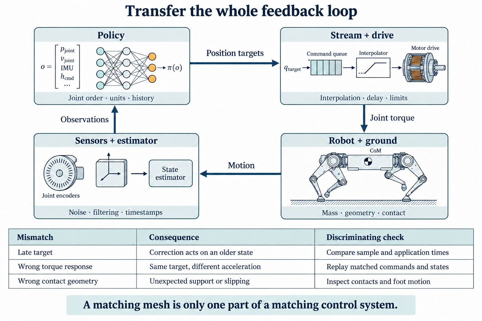
A robot dog learns in simulation by trying actions and observing what happens. For that experience to be useful on hardware, the simulated robot needs to respond like the real one: a joint target should produce comparable motion, a shift of body weight should produce comparable loading, and a correction should arrive at the right time.

The difference between those responses is the sim-to-real gap. Reducing it makes simulation a more useful place to design controllers, compare ideas and prepare for transfer.

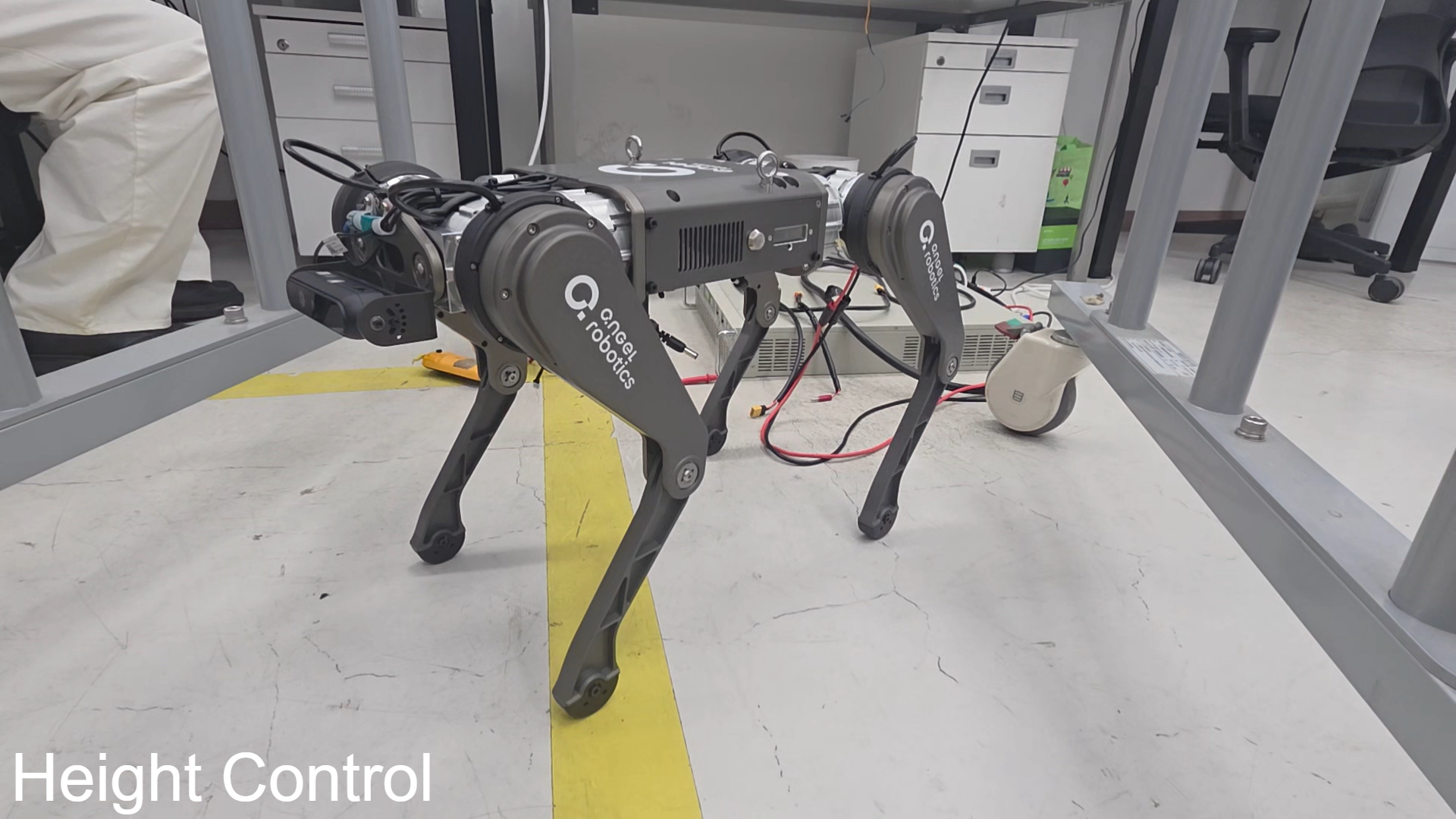
For our Angel D01 quadruped, the process starts with real experiments. We combine suspended-leg recordings, ground-supported poses, CAD and firmware information to build a model around the robot’s measured behaviour. System identification connects those measurements to model parameters; domain randomisation prepares a controller for a chosen range of variation around that model.

1. Begin with the whole control loop

A robot model includes more than dimensions and mass. D01 receives position commands, which pass through a target stream, the motor controller and a transmission before moving a joint. Encoders and other sensors report the resulting motion.

We therefore align three parts together:

Mechanics: joint geometry, mass distribution, rotational inertia and contact shapes.
Actuation: how position error and motion become current and joint torque, including limits and transmission ratios.
Information and timing: what the controller observes, when samples arrive and how targets change between updates.

This approach follows an important result from Tan et al., RSS 2018: combining system identification, actuator and latency modelling, and randomisation enabled transfer of learned quadruped locomotion. Their experiments showed that actuator behaviour and latency materially affected transfer. Read the paper.

For D01, we start by putting every signal into a consistent coordinate system. The measured flange angle becomes a model joint angle through

q_{joint} = s \frac{θ _{flange}}{r} + q_{0},

where

s

is the direction,

r

the external reduction and

q_{0}

the zero offset. Position targets use the same mapping; velocities use its scale and sign. This makes a recorded movement and its simulated replay refer to the same physical motion.

2. Two experiments reveal different parts of the robot

The central idea in our identification workflow is to separate leg gravity effects from whole-body support. The suspended and ground experiments complement each other.

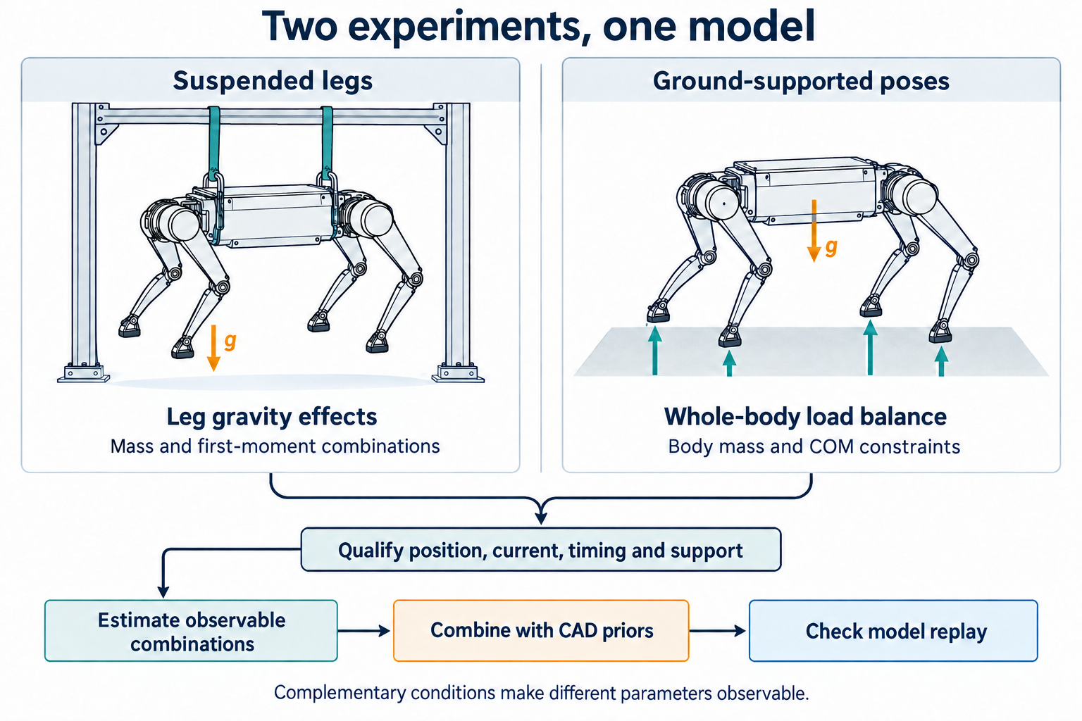
Suspended-leg measurements reveal leg gravity effects; ground-supported poses add body load-balance constraints. Qualified recordings and CAD priors feed a model checked by replay. — Suspended and ground-supported experiments expose different parts of the mechanics. Combining them gives the identification process more information.

Suspend the body to study the legs

With the torso supported and the feet clear of the floor, we can move a leg through different configurations without foot-ground forces entering its dynamics. Our recordings include controlled position trajectories, settled holds and the responses between them.

At a settled pose with a nearly stationary torso, velocity and acceleration terms become small. The gravity model predicts the joint torque required to support the leg; we compare that prediction with current-derived torque under explicit conversion and support assumptions. Bend the leg differently and the lever arms change, creating a different relationship between joint torque and mass distribution.

Think of holding a weight close to your elbow, then farther away. The weight is unchanged, but the effort needed to hold it increases. Sampling several leg configurations uses that same principle to reveal how mass is distributed along the links.

The same leg pose can require different effort when the body tilts, because gravity changes direction relative to the links. Body orientation therefore belongs in the gravity model.

Put the feet on the ground to study load balance

Ground-supported experiments add a new source of information: the legs now support the torso. The identification recordings include changes in body height and orientation while the feet support the robot.

Angel D01 standing on the laboratory floor during a body-height experiment. — D01’s ground-supported pose experiments connect joint loading with whole-body balance.

In a two-stage identification method, the leg parameters from the suspended fit are held fixed while estimating body mass and first moments. Ground forces connect the legs to the body’s weight: in a settled pose, both forces and moments balance. Different supported poses add constraints on body mass and centre of mass (COM).

Our constrained analysis searches for foot forces compatible with joint loading and whole-body equilibrium. Several load distributions can satisfy those equations, so we compare how well each model can explain the loading under stated contact and friction assumptions. The forces are inferred rather than measured by force plates. Four feet need not each carry a quarter of the weight.

3. Identify the parameters that change the response

System identification connects observed effort and motion to the mechanics that produce them. Each parameter answers a different physical question.

Parameter	Why it matters	What constrains it
Mass $m$	Weight and the force needed to accelerate a body	Supported loading, torque scale and mass priors
Centre of mass $c$	Gravity lever arms and how weight loads the legs	Suspended poses and whole-body equilibrium
Rotational inertia $I$	Resistance to angular acceleration	Informative moving trajectories, with reliable torque and timing
Geometry and joint coordinates	Foot placement and torque lever arms	CAD, dimensions and joint-coordinate checks
Current-to-torque conversion	How much joint effort a command produces	Motor/transmission definitions and independent torque references
Actuator response and delay	When and how strongly a correction acts	Commands and measured responses across different motions
Contact shape, friction and compliance	Support location, slip and impact response	Geometry and contact-sensitive experiments

For D01, the suspended/ground identification method concentrates on mass and COM. Geometry and joint mappings provide the fixed mechanical framework; firmware defines the actuation structure. These sources complement the quantities inferred from loading.

Mass and COM appear together in gravity torque

For a rigid link, its first mass moment is

h = m c, c = \frac{h}{m} .

Here

m

is in kilograms,

c

in metres and

h

in kg·m, expressed in a specified link frame. Gravity depends on both the amount of mass and its lever arm. Using first moments makes the gravity model linear in its unknown parameters:

τ_{g} = Y_{g} (q, R) θ .

The joint angles

q

and body orientation

R

determine the matrix

Y_{g}

;

θ

collects masses and first moments. Each suspended pose supplies another relationship between loading and mass distribution.

The mass model groups the robot into hip, thigh, calf assembly and trunk, sharing leg parameters through symmetry. Each group contributes

m, h_{x}, h_{y}, h_{z}

. Its equations distinguish six leg gravity combinations, with ground equilibrium adding total-mass and trunk-moment information under suitable pose variation.

One example from the suspended model is

β = h_{thigh, z} - ℓ_{thigh} m_{calf} .

This combination captures a thigh first moment together with the calf mass acting through the thigh length. Several anatomical parameter choices can produce the same

β

. The experiment estimates the gravity effect; CAD and mass priors help assign it to individual bodies. This is why a table of physical parameters can contain both data-informed estimates and retained priors.

Prior-regularised least squares combines the measured loading with this mechanical prior information:

\hat{θ} = θ ar g min ∥ A θ - b ∥_{2}^{2} + α ∥ D^{- 1} (θ - θ_{0}) ∥_{2}^{2} .

Here

A θ = b

stacks the pose-dependent loading equations,

θ_{0}

contains prior values, and the diagonal matrix

D

gives parameter scales in their corresponding units. The positive weight

α

sets the strength of the prior. The first term matches observed effort; the second stabilises parameter directions that the poses constrain weakly.

Ground support adds whole-body information

For a settled robot supported only by its feet, force and moment equilibrium give

i \sum f_{i} + M g = 0, i \sum (p_{i} - o) \times f_{i} + (c_{G} - o) \times M g = 0.

All vectors are in one common frame:

f_{i}

is a ground reaction,

p_{i}

its contact point,

M

total mass,

g

gravitational acceleration,

c_{G}

whole-robot COM and

o

the moment origin. Joint loading connects to those forces through

τ = τ_{g} - i \sum J_{i}^{T} f_{i},

where

J_{i}

maps joint motion to contact-point motion. The transpose maps a contact force back to joint torque. With leg gravity effects established, these equations constrain the trunk’s contribution. Changing supported poses changes the constraints; body tilt is especially relevant to resolving vertical COM information.

Motion reveals what static holds cannot

For a suspended leg with its base fixed, the rigid-body equation is

M (q) \overset{q}{¨} + C (q, \overset{q}{˙}) \overset{q}{˙} + g (q) = τ .

Here

M (q)

is the joint-space inertia matrix,

C (q, \overset{q}{˙}) \overset{q}{˙}

captures velocity-dependent effects, and

g (q)

is gravity torque. A settled hold mainly reveals

g (q)

. Accelerating the leg reveals inertia-dependent effort. Rotational inertia therefore needs dynamic excitation, while static loading constrains mass and COM combinations. Matching the experiment to the parameter is what makes the estimate useful.

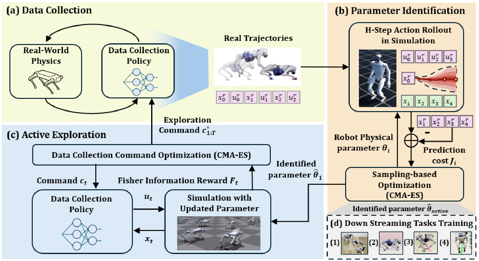
The same principle motivates SPI-Active, CoRL 2025. It identifies model parameters from multistep trajectory prediction and chooses additional commands to increase the information in the collected data. Its active exploration makes clear why the diversity of an experiment matters as much as the number of samples. Read the paper.

SPI-Active alternates parameter identification with informative exploration. — SPI-Active links model identification with informative experiments. Figure 2, Sobanbabu et al., CoRL 2025, CC BY 4.0. Cropped from the paper; figure unchanged.

4. Put the findings into a mechanically consistent model

A fitted number becomes useful when it describes the same body, frame and units as the simulator. Mass properties must match the bodies represented in the URDF—the file defining the robot’s links and joints. CAD and assembly geometry help place each mass and COM in the correct frame.

For example, a calf assembly may include a foot, while the URDF represents calf and foot separately. Their combined first moment must be preserved:

m_{assembly} c_{assembly} = m_{calf} c_{calf} + m_{foot} c_{foot} .

All positions in this equation must first be expressed in the same frame. For D01’s calf links, original CAD centroid coordinates provide the geometric basis for the COM choice, while the separate feet retain their own mass. Motor allocation and inertia transformations receive the same bookkeeping checks.

Physical checks include positive masses, plausible COM locations, valid inertia tensors and the correct total. Wensing, Kim and Slotine’s work on physically consistent identification formalises constraints on mass moments and bounding volumes, providing a principled way to connect fitting with realizable mechanics. Read the paper.

Contact geometry matters just as much as visual geometry. In our replay comparisons, using CAD-based calf collision shapes restored support at the feet while preserving suspended motion. A realistic contact surface lets the simulator apply forces at the right places, with the right lever arms.

5. Match the motors and clocks

The rigid-body model answers, “What motion follows this torque?” The actuator model answers, “What torque follows this command?” Both are needed.

In D01’s sampled current-domain implementation, the position error is expressed at the motor flange. With the integral and observer terms disabled, the core law is

e_{k} = θ_{k}^{*} - θ_{k}, i_{k} = clip (K_{p} e_{k} + K_{d} \frac{e _{k} - e _{k - 1}}{Δ t}, - i_{m a x}, i_{m a x}) .

K_{p}

has units A/rad and

K_{d}

has units A·s/rad. The sampled error difference includes changes in the target, so target interpolation affects the effort. We retain the hardware gains and represent limits, interpolation and delay explicitly.

For a sign-aligned motoring conversion, the joint torque is modelled as

τ_{joint} = s r η κ i,

where

κ

is flange torque per ampere,

r

the external reduction,

η

its efficiency and

s

the coordinate sign. An internal gear ratio already included in

κ

must not be applied again. This scale matters for identification too: changing the assumed torque per ampere changes the mass needed to explain the same current.

A useful research example is Hwangbo et al., Science Robotics 2019. They combined rigid-body simulation with a learned actuator model using histories of position errors and velocities to predict torque. Modelling that subsystem helped transfer learned behaviour to ANYmal. The practical lesson for D01 is to give actuator response its own explicit place in the simulator. Read the paper.

Timing is equally tangible. Imagine balancing a tray: it keeps moving between the moment you notice a tilt and the moment your correction takes effect. The robot also acts on a state that has evolved during sensing, computation and communication.

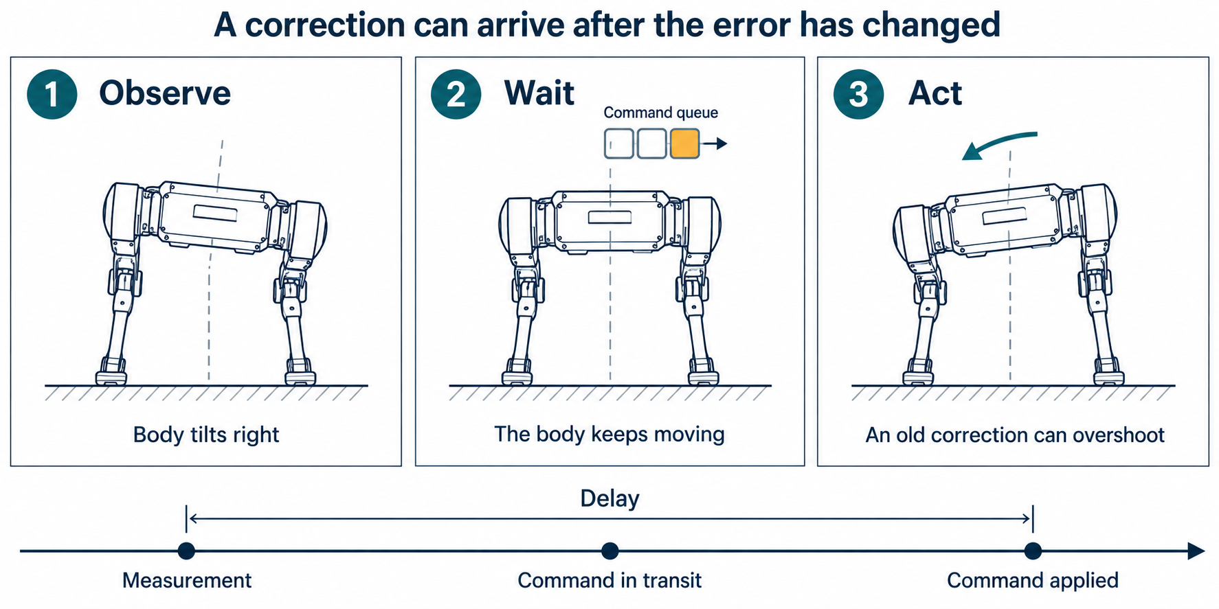
Observe a body tilt, wait while the body moves, then apply the earlier correction. — Delay changes when a correction acts. Matching the sensing, command and actuator clocks helps reproduce the same response.

At 10 Hz, a 20 ms delay occupies one fifth of a cycle: 72 degrees of phase lag. At 1 Hz, it occupies only one fiftieth: 7.2 degrees. The faster the motion, the more it changes during the same wait.

Explore delay, gain and frequency

A pure delay

d

adds

360 fd

degrees of phase lag to a sinusoid of frequency

f

, with

d

in seconds. This demo compares two first-order responses to the same repeating command. Increase delay to shift a response later, frequency to shorten the cycle, or gain to change its size.

Open the interactive illustration.

6. Replay the evidence and compare fairly

We connect the model back to the recordings in stages. Kinematic replay checks joint order, signs, offsets and pose reconstruction. Dynamic replay adds the drive law, mass properties, timing and support conditions, then compares predicted and recorded responses.

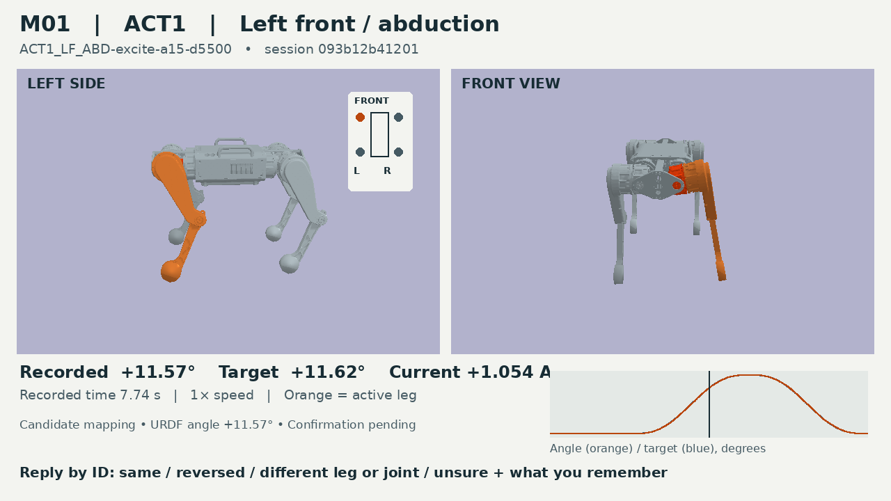
Recorded D01 joint positions reconstructed as a simulated robot pose. — Kinematic replay makes the recorded joint coordinates visible as a robot pose—the first layer of a replay check.

To test whether a model is better, replay the same commands from matched initial conditions and compare its predictions with real responses. Use separate validation motions to check whether the improvement carries beyond the fitting conditions.

The measurements follow the question: position tracking for motion, torque/current compatibility for loading, timing sensitivity for actuation, and contact locations for support. For stationary standing, we also measure body tilt, accumulated foot travel, drift, recovery and effort under a defined disturbance envelope. Planted balance and stepping recovery are evaluated as distinct behaviours.

A practical lesson from our comparisons is to inspect every joint as well as the average: a lower total fitting error can redistribute error among axes. Loading, motion and contact each test a different part of the model.

7. Use domain randomisation around the evidence

Even a carefully constructed model represents a range of real conditions. Dynamics randomisation trains across variations in quantities such as mass distribution, actuator response, delay, sensor noise and contact. The controller learns to handle a family of plausible robots and environments.

Peng et al., ICRA 2018, demonstrated this on a robotic-arm pushing task, varying physical parameters, action timing and observation noise. The method complements identification: identification locates a useful nominal model; randomisation prepares the controller for variation around it. Read the paper.

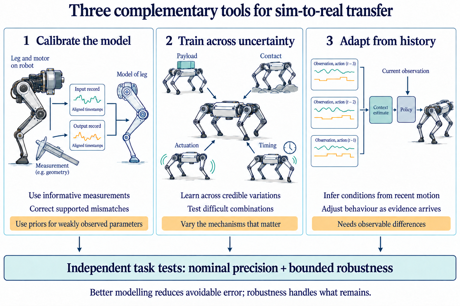
Calibration uses measurements, randomisation covers plausible variation, and adaptation uses motion history to infer context. — Identification, randomisation and adaptation play complementary roles. Adaptation uses past state/action information alongside the policy’s current observations.

Reducing the gap still matters because it gives randomisation a meaningful centre and structure. A delayed actuator is best represented with a delay mechanism; a payload changes mass, COM and inertia together. Evidence helps us choose variations that correspond to the robot and preserve these relationships.

Adaptation can add another layer. RMA, RSS 2021, uses recent state/action history to infer context for its policy, allowing behaviour to adjust to changing conditions. This is a useful extension when deployment conditions vary. Read the paper.

For D01, the foundation is the experiment-to-model loop: choose a condition that reveals something useful, relate loading and motion to physical parameters, preserve mechanical consistency and check the resulting response. That is how real data makes simulation more useful—and how a better simulator supports the next controller design.